The 1993 answer was right until it wasn't

If you ship things, or move electricity, or route data, you eventually meet the multi-commodity flow problem. You have a network with limited capacity on each link, and a long list of things that need to get from somewhere to somewhere else. Everything competes for the same capacity. Find the cheapest way to satisfy all of it at once.

The problem is old and well understood. What is less well understood is that there is more than one way to write it down, and the choice matters enormously.

Two ways to describe the same thing

You can describe a solution as a set of paths: this shipment goes A→C→F, that one goes B→C→G. Natural, and it is how most people would sketch it on a whiteboard.

Or you can describe it as a set of trees: everything leaving source A, considered together, forms a shortest-path tree fanning out across the network. Instead of one description per shipment, you get one per origin.

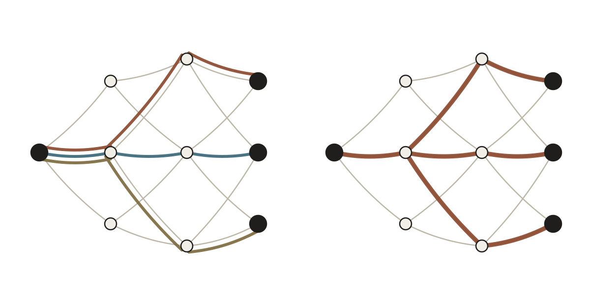
That distinction sounds academic until you count. A logistics network might have a few hundred origins and several million individual shipments. The path-based description needs a row in its bookkeeping for every shipment. The tree-based one needs a row for every origin. Same problem, same answers, wildly different amounts of paper.

Why the question was closed

In 1993, Jones, Lustig, Farvolden and Powell compared the two properly. They found the path-based version converged in fewer rounds and finished faster in wall-clock time. Fewer rounds and less time is not a close call. The question was settled, and the answer was inherited by everyone downstream for thirty-two years.

Their measurement was correct. I want to be clear about that, because the interesting part is not that they were wrong.

What changed

We re-ran the comparison on 44 instances, the largest with 3.3 million commodities, about a thousand times the scale available in 1993.

The convergence finding held up exactly. The tree-based formulation still needs two to three times as many rounds. If you count rounds, 1993 is still right.

The wall-clock finding reversed under every solver we tried: five different linear-programming backends, open-source and commercial, CPU and GPU. Tree-based came out 1.4 to 1.9 times faster on average, and 99 times faster on the largest instance. It also finished 43 or 44 of the 44 instances, where path-based managed 38 to 42, and its failures clustered exactly where you would least want them, on the biggest problems.

Why, and why it took thirty-two years

Measurement tells you what happened; it does not tell you why. So we measured the inside too.

The master problem, the bookkeeping step that reconciles everything, turned out to be 87 to 99 percent of the total runtime on three of our four instance families. Almost nothing else matters there. And the tree-based master is up to 32 times smaller at the point it finishes.

The fourth family is the exception that says what the mechanism is. On the intermodal instances the master is a fifth of the runtime or less, sometimes one percent, and the pricing step is where the time goes. Those instances have one commodity per source, so a tree is a path, the tree-based master has exactly the same number of rows as the path-based one, and there is nothing to compress. They neither gain nor lose.

So the tree-based method takes more rounds, but each round is against a far smaller object. In 1993, at the scale then reachable, the extra rounds dominated. At three orders of magnitude more scale, the size of the thing you carry through each round dominates instead. The crossover was always there. Nobody had a machine big enough to walk past it.

Iterations were the wrong thing to count. They were a reasonable proxy for time when the objects were small, and they stopped being one when the objects grew.

The case where it loses

We also published the case where our method loses. On one instance, planar2500, where the number of origins approaches the number of nodes, the tree-based version is eight times slower, and for a comprehensible reason: a tree column then touches most of the master’s rows, so the smallness that made it fast is gone.

Publishing the counterexample is not modesty. It is the thing that makes the rest of the numbers worth believing. It also tells you exactly when to use this and when not to, which is what anyone deciding whether to adopt it actually needs.

An objection

After the paper went out, it was pointed out to me that there is an approximation scheme for this, and that it is much faster. Read the congestion off the edges, update the edge costs from it, reroute by shortest paths, repeat. There is no master problem in it at all, which is not a trick: it is simply a different method, and nothing is being reconciled centrally, so there is nothing for a master problem to do.

What it gives up is exactness. Column generation returns an optimum with valid dual values. An approximation scheme returns something within a tolerance you choose. At the sizes where any of this matters, that is very often a trade worth making, and I would not claim otherwise.

The part I would want a reader to keep

Older results are not wrong so much as scoped. The scope is usually invisible, because it lives in the hardware available when the measurement was taken. It is worth asking, occasionally, which of the things you know were settled on machines a thousand times smaller than the one on your desk.

The paper is arXiv:2509.24656, with Bjørn Petersen, and the implementation is at mcfcg.